Exformation & Logical Depth

"!"

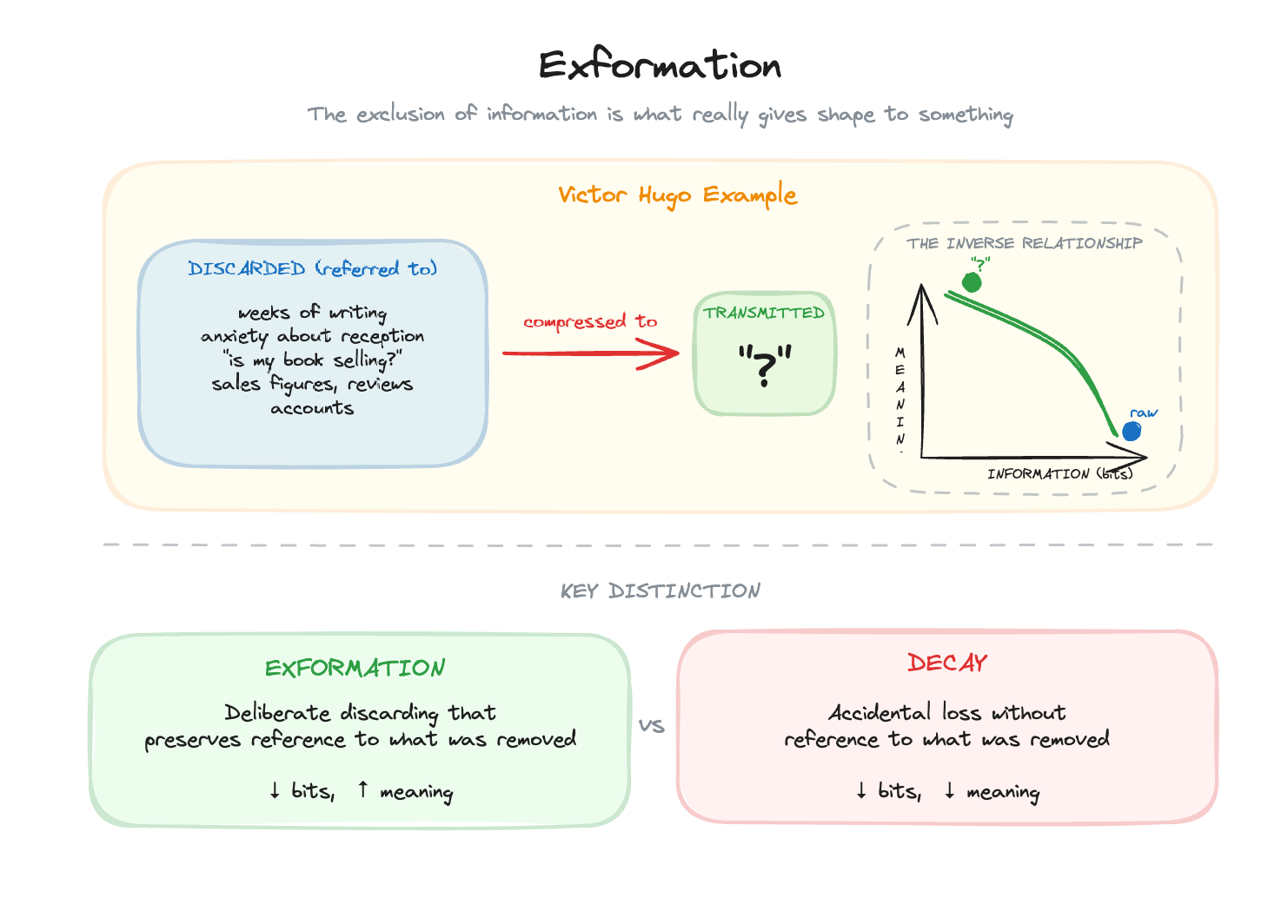
After submitting Les Misérables to his publisher, Victor Hugo went on holiday. Anxious to know how the book was selling, he sent a telegram containing only: “?”

His publisher replied: “!”

One character sent. One character received. Yet the exchange carried everything Hugo needed to know, weeks of writing, the anxiety of reception, sales figures, critical response, all compressed into a single symbol.

Tor Nørretranders calls this exformation: “Information is interesting once we have got rid of it again: once we have taken in a mass of information, extracted what is important, and thrown the rest out.”¹

More precisely, exformation is “explicitly discarded information. Not merely a discarding of information: He has not simply forgotten it all. He refers explicitly to what he has discarded.”²

This is also what a good data model does. The value of a well-structured warehouse isn’t the data it contains; it’s the data that was filtered, reconciled, and thrown away to arrive at what remains. The ingenuity is in the discarding.

The problem is that discarding can be meaningful or destructive. Exformation creates value. Decay destroys it. Both look like data reduction. How do you tell the difference?

Why Consciousness Uses Exformation

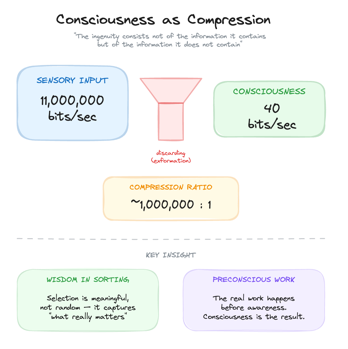
The concept comes from his investigation into how consciousness works.

Our sensory systems take in approximately eleven million bits per second. Our conscious awareness processes about forty bits per second. That’s a ratio of roughly a million to one. As Nørretranders summarises: “Only one millionth of what our eyes see, our ears hear, and our other senses inform us about appears in our consciousness.”³

This exclusion of information is necessary.

Consciousness cannot process everything, it must discern. The question is whether that selection is random or meaningful. Nørretranders: “There must necessarily be a degree of ‘wisdom’ in the sorting that takes place, otherwise we would just go around conscious of something random, with no connection to what really matters.”⁴

Here’s the key line: “Consciousness is based on an enormous discarding of information, and the ingenuity of consciousness consists not of the information it contains but of the information it does not contain.”⁵

The value is in the discarding. Consciousness is ingenious because it knows what is important. But, and this is critical, the sorting and interpretation required for it to know what is important is not itself conscious. The real work happens before awareness. Consciousness is the result of exformation, not the process that produces it.

Why does this matter for data modelling?

This maps directly onto data modelling. A well-structured warehouse isn’t valuable because of the data it contains. It’s valuable because of what was removed, filtered, reconciled, and compressed to arrive at what remains. The ingenuity is in the discarding.

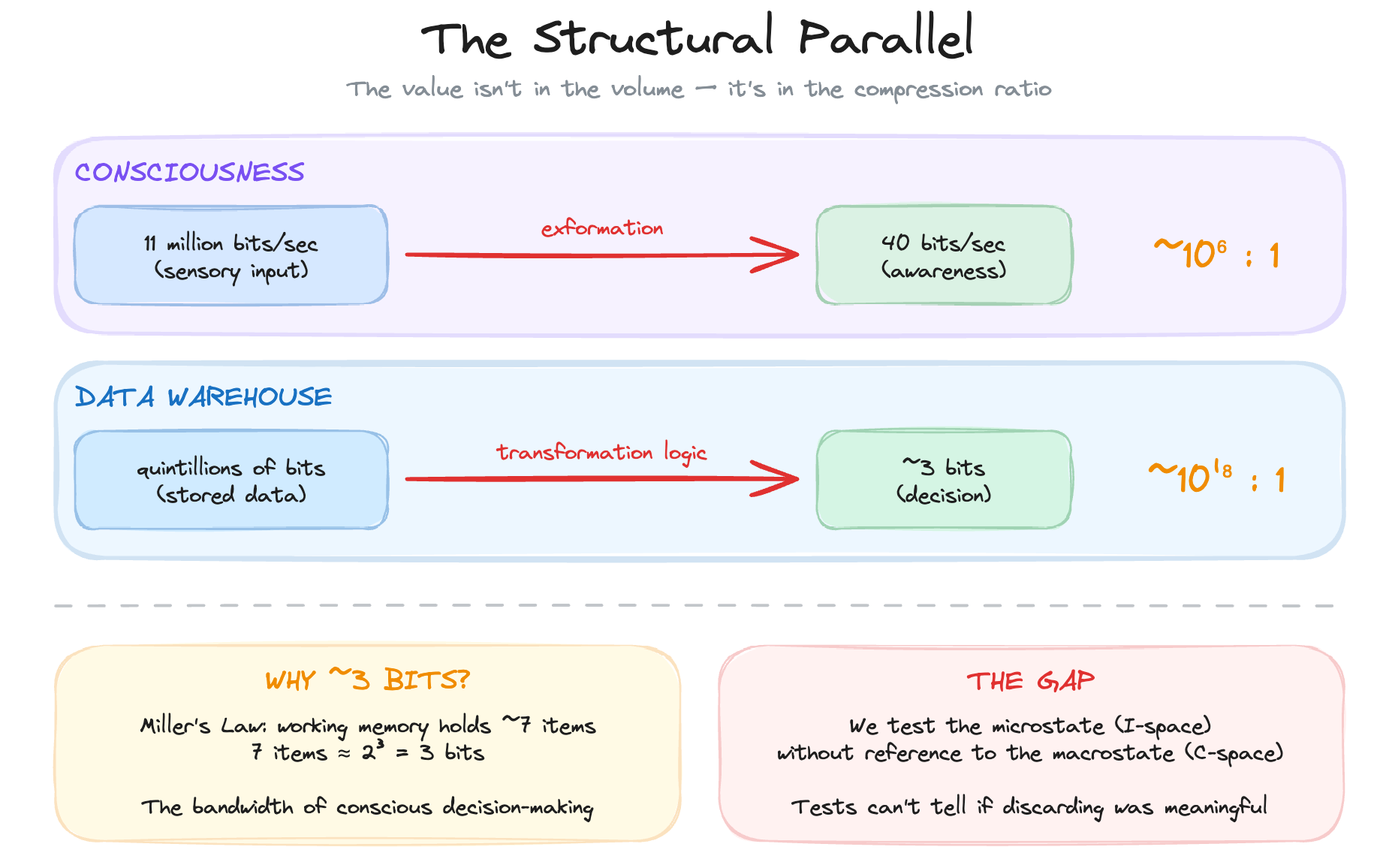
There are quintillions of bits of information in a modern data warehouse. There’s no way that a person can make use of that without the selection and filtering of records. A data model selects what’s important and this hinges on the desired macrostate, ontology and goals of the institution that consumes it. The role of a data model is to get those quintillions of bits of information crunched down to as close to the 3 bits of information required to make a decision as possible.

Why three bits? Miller’s Law tells us that conscious working memory holds about seven items.⁶ Seven items represents just under three bits of information (since 2³ = 8). That’s the bandwidth of conscious decision-making, the bottleneck through which all action must pass. The idea of a great analytics system is to compress huge amounts of information into the smallest possible tokens, to get from quintillions to three.

So the parallel is structural:

• Consciousness: 11 million bits/sec in → 40 bits/sec out

• Data warehouse: quintillions of bits stored → ~3 bits to decide

In both cases, the value isn’t in the volume. It’s in the compression ratio. It’s in the computational work that selects, filters, and discards to arrive at what matters. Nørretranders draws an analogy to money: “Information and meaning are rather like money and wealth. Real value, real wealth, is a matter not of money but of the money you have spent, money you used to have: utility values you have obtained by paying for them.”⁷

The value isn’t in the bits you store. It’s in the bits you’ve processed and discarded to arrive at what remains. A dashboard showing three KPIs is valuable precisely because of the quintillions of bits that were filtered, aggregated, validated, and thrown away to produce those numbers.

A discoverable data warehouse saves you costs precisely because of the information it doesn’t contain. The reduction of noise means that the information available, and its inferable shape, reduces the need for additional dimensionality. You structure implicit meaning into the data by removing what doesn’t belong. Not only does this impose more meaning, it decreases storage and query costs.

This is what transformation logic does. Every CASE statement, every JOIN, every aggregation discards information. The question is whether that discarding is deliberate and meaningful (exformation) or accidental and destructive (decay).

The structural problem is that we don’t currently test for this.

The standard tests in data pipelines, uniqueness, cardinality, null checks, referential integrity are test properties of I-space in isolation. Are there duplicates? Are foreign keys valid? Is this column populated? These are necessary. But they can’t tell you if the discarding was meaningful or anything about the semantic coherence of the output.

A table can pass every test and still be semantically wrong. Every row unique, every foreign key valid, every column populated, and yet the data doesn’t represent what it claims to represent. The tests check the shape of the output, not the quality of the compression that produced it.

We test the microstate without reference to the macrostate. We measure I-space properties without asking whether they align to C-space expectations.

Computation as Discarding

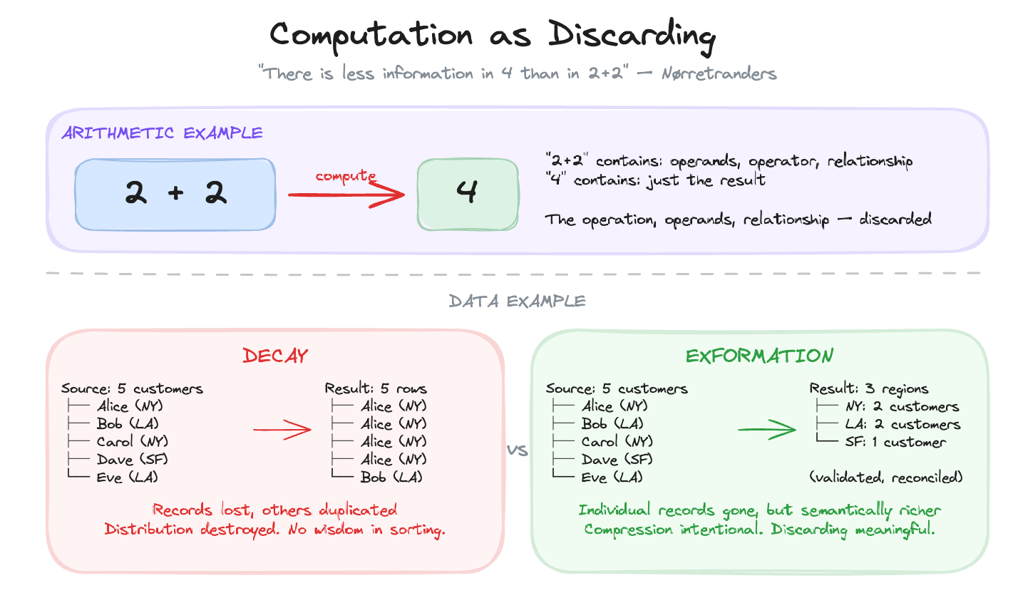
Nørretranders: “Computation is a process in which information is discarded. Something real, irrevocable, and irreversible takes place... There is less information in 4 than in 2+2.”⁸

Think about that. The expression “2+2” contains more information than “4”. It specifies the operation, the operands, the relationship. When you compute the result, you discard all of that. What remains is simpler, but it carries the meaning of what was lost.

The same is true for transformation logic. Every dbt model, every SQL transformation, every data pipeline is a computation that discards information. The curation of information and the removal of redundancy is where the real work happens, and that work has a cost.

Sipser, in Introduction to the Theory of Computation, poses the central question of complexity theory: “What makes some problems computationally hard and others easy?”¹⁹ In data modelling, the answer is bound up with discarding. The hard problems are those where meaningful compression is difficult, where you can’t easily separate signal from noise, where the “wisdom in the sorting” requires deep domain knowledge and careful design.

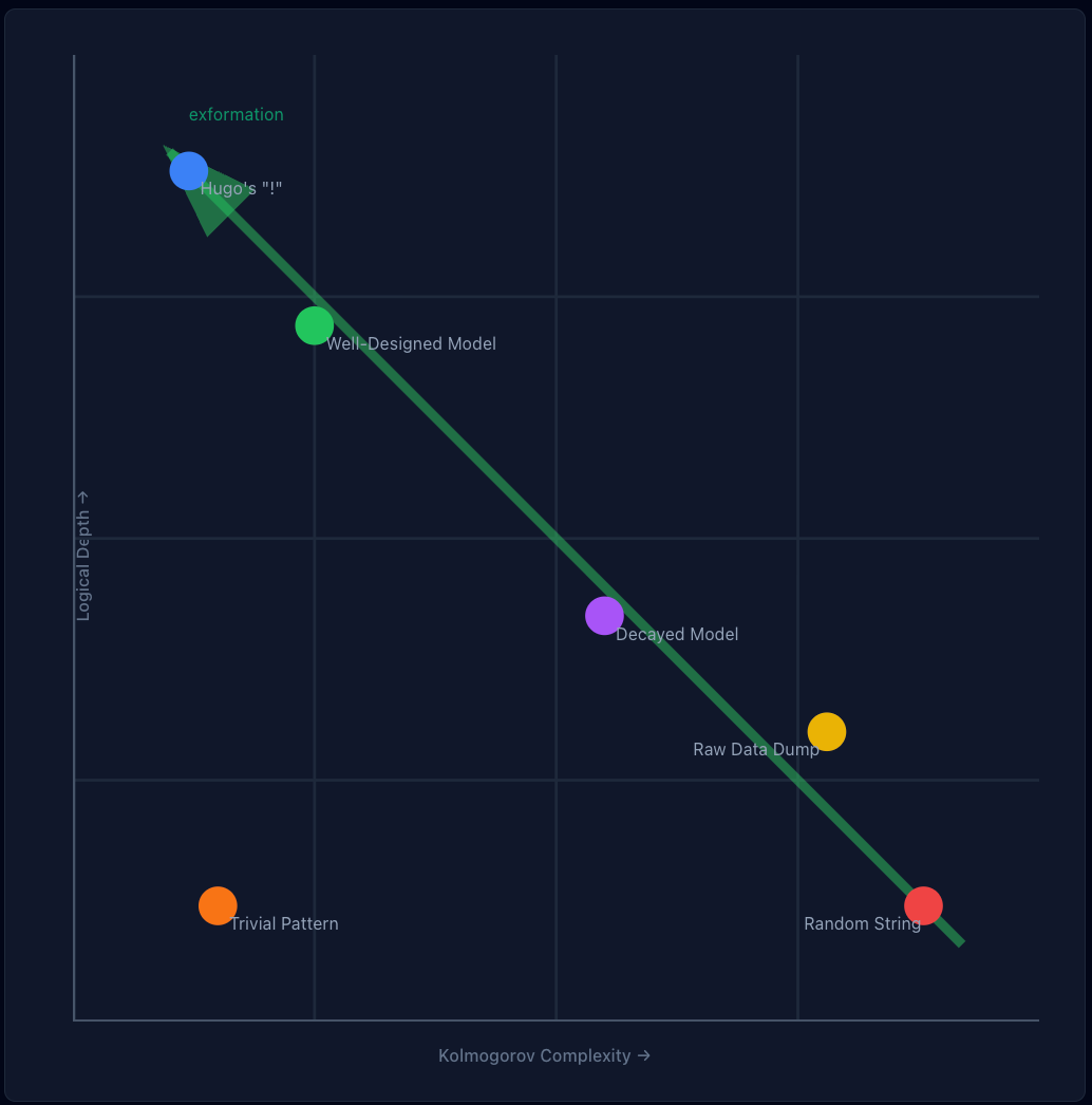
Consider a source system with five customer records, each with different attributes. After a poorly designed transformation, the warehouse shows the same customer duplicated four times with one original remaining. Records have been lost. Others have been duplicated. The distribution of the source is destroyed. This isn’t exformation, there’s no wisdom in the sorting. The meaning of the original data is gone. That’s decay.

A well-designed transformation, by contrast, might aggregate those five records into a single customer profile with validated, reconciled attributes. The individual records are gone, but what remains is semantically richer. The compression was intentional. The discarding was meaningful. That’s exformation.

Logical Depth

How do we distinguish meaningful compression from decay? This is where Charles Bennett’s concept of logical depth becomes essential.⁹

Bennett defines logical depth as the computational work required to generate an object from its shortest description, essentially the “computational history” embedded in a structure. Mitchell, in Complexity: A Guided Tour, summarises it: “Logically deep objects… contain internal evidence of having been the result of a long computation or slow-to-simulate dynamical process, and could not plausibly have originated otherwise.”¹⁰

This is what defines a well-ordered data model. It contains internal evidence of having been carefully constructed, you can tell the difference between a schema that emerged from thoughtful design and one that was thrown together.

This distinguishes between:

• Shallow objects: Random strings (high entropy, no history) OR trivial patterns like “AAAAAAA” (low entropy, minimal computation)

• Deep objects: Living organisms, crystals, meaningful data (may have any entropy level, but required significant computation to create)

Nørretranders interprets Bennett: “Logical depth is a measure of the process that leads to a certain amount of information, rather than the amount of information that is produced. Complexity or meaning is a measure of the production process rather than the product, the work time rather than the work result. The information discarded rather than the information remaining.”¹¹

Elsewhere he puts it more directly: “The logical depth of a message is the measure of its meaning, its value. The more difficulty the sender experiences in arriving at the message, the greater its logical depth. The more ‘calculating time’ he has spent, in his head or on a computer, the greater its value, as he saves the recipient the trouble of doing the work himself.”¹²

This connects to a broader point Nørretranders makes: “The complexity of the physical and biological world can be described as depth: the amount of discarded information.”¹³ The work of building a good data model is thermodynamically real, it requires energy to impose order on disorder.

This resolves something I noted in The Real and the Hard Problem of Data Modelling: perfect order can be perfectly wrong. A database where every age is 999 has low Shannon entropy but zero logical depth. It’s trivially ordered and no computational work validates it.

Real customer data might have high Shannon entropy (ages distributed across decades) but high logical depth (each record validated, transformed, reconciled against business rules).

It’s not that entropy level doesn’t matter, or that computational history doesn’t matter. You have to measure and consider both. As Cover and Thomas define it, “The entropy is a measure of the average uncertainty in the random variable. It is the number of bits on average required to describe the random variable.”²⁰ Logical depth is a proxy for semantic meaning. Statistical entropy is a measure of I-space order and surprise.

You need both axes.

Two Axes of Complexity

Kolmogorov complexity provides another lens. Cover and Thomas explain that “Kolmogorov, Chaitin, and Solomonoff put forth the idea that the complexity of a string of data can be defined by the length of the shortest binary computer program for computing the string. Thus, the complexity is the minimal description length.”¹⁴ This is algorithmic compression, how small can you make the program that generates this output?

Cover and Thomas explain: “There is a pleasing complementary relationship between algorithmic complexity and computational complexity. One can think about computational complexity (time complexity) and Kolmogorov complexity (program length or descriptive complexity) as two axes corresponding to program running time and program length.”¹⁵

Kolmogorov complexity and computational complexity are two different axes. One measures program length (how compact the description). The other measures running time (how much work to execute). Logical depth lives on the second axis. It’s not about how short your description is. It’s about how much computation is embedded in the result.

A random string has high Kolmogorov complexity, you can’t compress it, so you need a long program to reproduce it. But it has zero logical depth, no computational history, no work invested. A well-designed data model has the inverse property: potentially low Kolmogorov complexity (the schema is compact and elegant) but high logical depth (significant computational work validates every record).

This connects to Occam’s Razor. As Cover and Thomas put it, citing William of Occam: “Causes shall not be multiplied beyond necessity,” or to paraphrase, “The simplest explanation is best.”¹⁶ In data modelling terms, the simplest schema that adequately represents the business is best. But simplicity in description doesn’t mean simplicity in production. The most elegant models often require the most work to create, which is precisely what logical depth measures.

Lloyd proposed three dimensions for measuring complexity: How hard is it to describe? How hard is it to create? What is its degree of organisation?¹⁷ These map directly onto data modelling concerns and provide a way to measure the effectiveness of a model. A good model should be easy to describe (semantic clarity), hard to create (high logical depth from the computational work invested), and highly organised (ontological coherence).

As Mitchell puts it: “A model, in the context of science, is a simplified representation of some ‘real’ phenomenon... Models are ways for our minds to make sense of observed phenomena in terms of concepts that are familiar to us.”¹⁸ A model exists to serve a purpose, not to show all information, but a curated subset that serves a specific goal. The curation is the value.

The inverse is the problem: a model that’s easy to create but hard to describe has low logical depth and high semantic entropy. It looks like data, but it doesn’t mean anything.

Measuring Logical Depth Requires a Target State

Bennett’s formal definition is precise, logical depth is the time required to execute the shortest program that produces an output. But here’s the catch, you can’t measure “time to produce” without knowing what you’re producing.

In data modelling terms, you can’t measure the computational work invested in reaching a state unless you’ve declared what that state should be.

This is what’s been missing. The transformation pipeline exists. The dbt DAGs exist. The CASE statements and window functions and reconciliation logic, all of it embeds computational history. But computational history toward what? Without a declared target state, you’re measuring effort without direction. You might have deep computation that produces the wrong thing. Or shallow computation that happens to produce the right thing by accident.

MML as the Macrostate

Modality’s MML is effectively the Kolmogorov complexity of your semantic intent, the shortest description of “what the data should look like.” It declares entities, attributes, relationships, classifications, derivations, and metrics. It’s compressed institutional logic.

With MML in place, you have both sides of Bennett’s equation:

• The minimal description: the MML model (what should exist)

• The computation time: the transformation pipeline (how long to get there)

Logical depth becomes measurable: the computational work required to transform source data into conformance with the declared MML specification.

What This Enables

• Coverage: How much of the declared model has implementation backing it?

• Depth per entity: How much transformation work validates each declared entity?

• Drift detection: When implementation diverges from declaration, logical depth becomes suspect

• Proof-of-work: The pipeline is evidence that computation occurred; MML is evidence of what the computation was for

The target state was always the missing piece. It lived in Confluence, in Lucidchart, and that’s if you were lucky. If you weren’t lucky, it lived in the engineer’s head who’s currently on the last week of their notice period.

Now it lives in code. Version-controlled, diffable, executable.

You can finally start to answer how much computational work validates this data against the semantic structure we intended?”

What’s Coming?

The standard tests in data pipelines, uniqueness, null checks, and referential integrity, verify properties of the output. They can’t tell you whether the discarding that produced that output was meaningful.

A table can pass every test and still be semantically wrong. Every row is unique, every foreign key is valid, and every column is populated and yet the data doesn’t accurately represent what it claims to represent. The tests check the shape of the result, not the quality of the compression that created it.

This is what logical depth gives us. A way to distinguish between structure that emerged from meaningful work versus structure that emerged by accident. But Bennett’s definition requires knowing what you’re producing. You can’t measure computational depth toward a target state you never declared.

That’s what MML provides. The target state, what the data should look like, now lives in code. With it in place, you can finally ask, ‘How much computational work validates this data against the semantic structure we intended?’.

The next article will show how to measure that and how that measurement enables the use of genetic algorithms as part of your modelling approach.

---

Notes

1. Nørretranders, T. (1998). *The User Illusion: Cutting Consciousness Down to Size*. Viking Press, p.221.

2. Nørretranders, *The User Illusion*, p.106.

3. Nørretranders, *The User Illusion*, p.140.

4. Nørretranders, *The User Illusion*, p.187.

5. Nørretranders, *The User Illusion*, p.187-188.

6. Miller, G.A. (1956). “The Magical Number Seven, Plus or Minus Two: Some Limits on Our Capacity for Processing Information.” *Psychological Review*, 63(2), pp.81-97. See also Nørretranders, *The User Illusion*, p.146: “Symbols are the Trojan horses by which we smuggle bits into our consciousness.”

7. Nørretranders, *The User Illusion*, p.112.

8. Nørretranders, *The User Illusion*, p.119.

9. Bennett, C.H. (1988). “Logical Depth and Physical Complexity.” In Herken, R. (ed.), *The Universal Turing Machine: A Half-Century Survey*. Oxford University Press.

10. Mitchell, M. (2009). *Complexity: A Guided Tour*. Oxford University Press, p.107.

11. Nørretranders, *The User Illusion*, p.92-93.

12. Nørretranders, *The User Illusion*, p.92.

13. Nørretranders, *The User Illusion*, p.221.

14. Cover, T.M. & Thomas, J.A. (2006). *Elements of Information Theory*, 2nd ed. Wiley-Interscience, p.12.

15. Cover & Thomas, *Elements of Information Theory*, p.12.

16. Cover & Thomas, *Elements of Information Theory*, p.13, citing William of Occam.

17. Lloyd, S. (2001). “Measures of Complexity: A Nonexhaustive List.” *IEEE Control Systems Magazine*, 21(4), pp.7-8.

18. Mitchell, *Complexity*, pp.206-207.

19. Sipser, M. (2012). *Introduction to the Theory of Computation*, 3rd ed. Cengage Learning, p.25.

20. Cover & Thomas, *Elements of Information Theory*, p.19.

---

This article is part of a series leading to Modality, a data modelling tool that lets teams define, document, and govern their data models using MML (Modality Modeling Language). It puts data modelling and classification first instead of last, and helps business users, agents and engineers monitor the delta between a logical target state and the current state.